In this blog series, we’ll investigate the simulation of beams of ions or electrons using particle tracking techniques. We’ll begin by providing some background information on probability distribution functions and the different ways in which you can sample random numbers from them in the COMSOL Multiphysics® software. In later installments, we’ll show how this underlying mathematics can be used to accurately simulate the propagation of ion and electron beams in real-world systems.
The Motivation Behind Utilizing Probability Distribution Functions
Energetic beams of ions and electrons are a topic of great interest in the fundamental research of high-energy and nuclear physics. But they are also utilized in a wealth of application areas, including cathode ray tubes, the production of medical isotopes, and nuclear waste treatment. In the accurate computational modeling of beam propagation, the initial values of the particle position and velocity components are of particular importance.
When releasing ions or electrons in a beam for a particle tracing simulation, we’re often required to sample these particles as discrete points in phase space. However, before we delve too deeply into what phase space is and how ions or electrons fit into it, let’s learn more about probability distribution functions and how they can be utilized in COMSOL Multiphysics.
Introduction to Probability Distribution Functions
Let’s start with some definitions. A continuous random variable x is a random variable that can take on infinitely many values. For example, suppose that a point x1 is selected at random along a line segment of length L. Then a second point x2 is selected elsewhere along this line. Assuming that these two points are distinct, we can then select a third distinct point ![]() that is also on the line, then a fourth point
that is also on the line, then a fourth point ![]() , and so on, and thus infinitely many distinct points can be obtained. This is illustrated below.
, and so on, and thus infinitely many distinct points can be obtained. This is illustrated below.
![Image depicting distinct points on three lines.]()
As a side note, the other kind of random variable is called a discrete random variable and can only take on specified values. Think about flipping a coin or drawing a card from a deck; the number of outcomes is finite.
A 1D probability distribution function (PDF) or probability density function f(x) describes the likelihood that the value of the continuous random variable will take on a given value. For example, the probability distribution function
(1)
f(x) = \left\{
\begin{array}{cc}
0 & x\leq 0\\
1 & 0 < x < 1\\
0 & 1\leq x
\end{array}
\right.
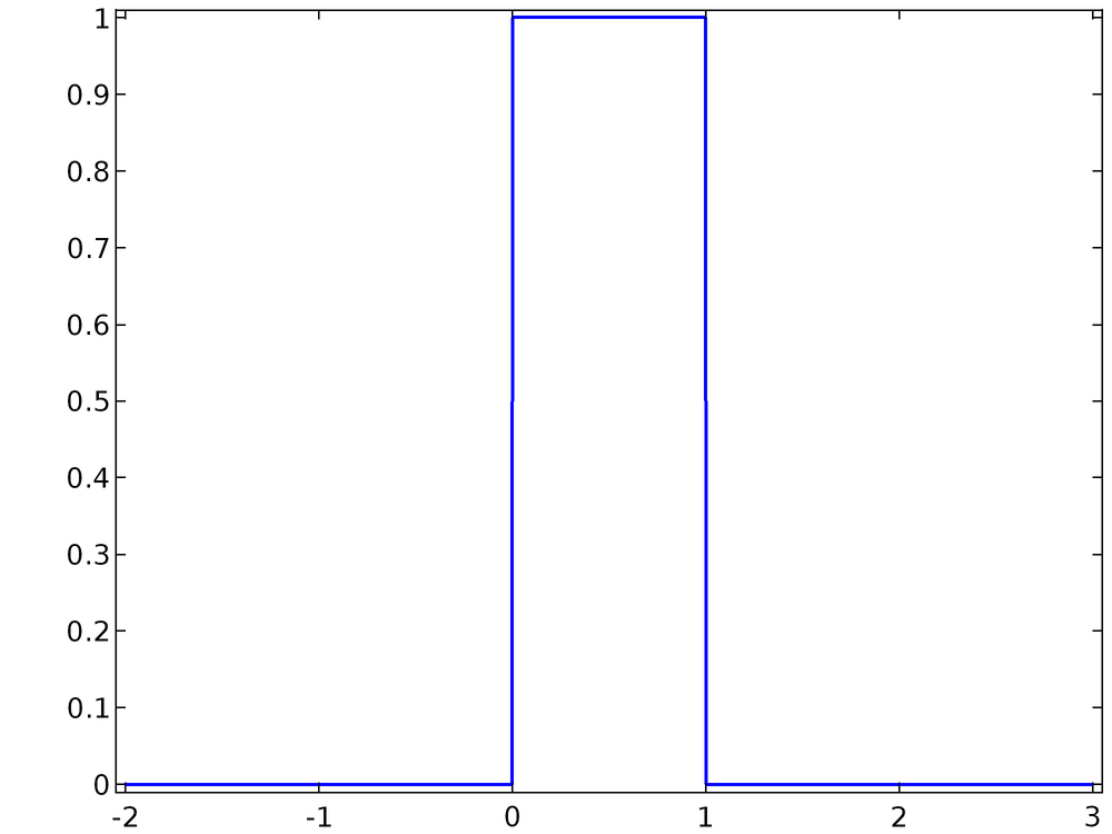
describes a variable x that has a uniform chance to take on any value in the open interval (0, 1) but has no chance of having any other value. This PDF, a uniform distribution, is plotted below.
![Plot depicting a uniform distribution.]()
Probability distribution functions can also be applied for discrete random variables, and even for variables that are continuous over some intervals and discrete elsewhere. An alternative way to interpret such a random variable is to treat it as a continuous random variable for which the PDF includes one or more Dirac delta functions. This blog series will only consider continuous random variables.
The PDF is normalized if
\int_{-\infty}^{\infty} f(x)dx = 1
In other words, the total probability that the variable x takes on a value somewhere in the range (-∞, ∞) is unity.
A cumulative distribution function (CDF) F(x) is the likelihood that the value of the continuous random variable lies in the interval (-∞, x). The PDF and CDF are related by integration,
F(x) = \int_{-\infty}^{x} f(x^\prime) dx^\prime
From the above definition, it is clear that if the probability distribution function is normalized, then
\textrm{lim}_{x \rightarrow \infty} F(x) = 1
The PDF from Eq.(1) and the corresponding CDF are plotted below. It is clear that the PDF, as written, is normalized.

Sampling from a 1D Distribution
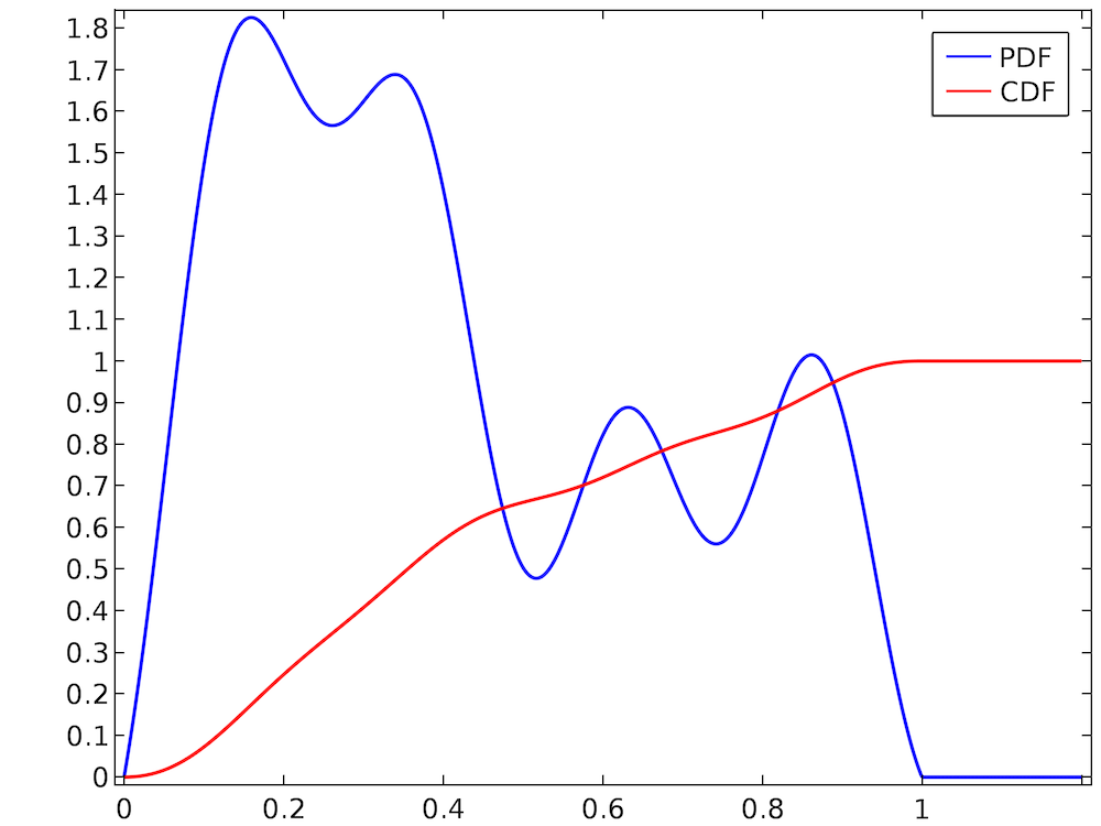
Selecting a value at random from a uniform distribution is usually quite easy. In most programming languages, routines to generate uniformly distributed random numbers are readily available. However, suppose that we have a much more arbitrary distribution like the one shown below.
![Graph showing an arbitrary distribution.]()
The random number takes on values in the interval (0, 1), and the PDF is normalized because the CDF ends up at 1. However, the distribution is clearly not uniform; for example, the random number is much more likely to be in the range (0.2, 0.3) than the range (0.7, 0.8). Simply using a built-in routine that samples uniformly distributed random numbers from the interval (0, 1) would not be correct. Therefore, we must consider alternative ways to sample random numbers from this arbitrary-looking PDF.
This brings us to one of the most fundamental methods for sampling values from a probability distribution function, inverse transform sampling. Let U be a uniformly distributed random number between zero and one. (In other words, U follows the distribution function given by Eq.(1).) Then to sample a random number with a (possibly nonuniform) probability distribution function f(x), do the following:
- Normalize the function f(x) if it isn’t already normalized.
- Integrate the normalized PDF f(x) to compute the CDF, F(x).
- Invert the function F(x). The resulting function is the inverse cumulative distribution function or quantile function F-1(x). Because we’ve already normalized f(x), we could also clarify by calling this the inverse normal cumulative distribution function, or simply the inverse normal CDF.
- Substitute the value of the uniformly distributed random number U into the inverse normal CDF.
To summarize, F-1(U) is a random number with a probability distribution function f(x) if ![]() . Let’s look at an example in which this method is used to sample from a nonuniform probability distribution function.
. Let’s look at an example in which this method is used to sample from a nonuniform probability distribution function.
Example 1: The Rayleigh Distribution
The Rayleigh distribution appears quite frequently in the equations of rarefied gas dynamics and beam physics. It is given by
(2)
f(x) = \left\{
\begin{array}{cc}
0 & x<0 \\
\frac{x}{\sigma^2} \exp\left(-\frac{x^2}{2\sigma^2}\right) & x\geq 0
\end{array}
\right.
where σ is a scale factor yet to be specified. We can verify that the Rayleigh distribution, as written above, is normalized,
\begin{aligned}
\int_{0}^{\infty} \frac{x}{\sigma^2} \exp\left(-\frac{x^2}{2\sigma^2}\right)dx
&= \lim_{x \rightarrow \infty} \left.-\exp\left(-\frac{x^\prime^2}{2\sigma^2}\right)\right|^x_0\\
&= 1-\lim_{x \rightarrow \infty}\exp\left(-\frac{x^2}{2\sigma^2}\right)\\
&= 1
\end{aligned}
The cumulative distribution function is
\begin{aligned}
F(x)
&=\int_{0}^{x} \frac{x^\prime}{\sigma^2} \exp\left(-\frac{x^\prime^2}{2\sigma^2}\right)dx^\prime\\
&= \left.-\exp\left(-\frac{x^\prime^2}{2\sigma^2}\right)\right|^x_0\\
&= 1-\exp\left(-\frac{x^2}{2\sigma^2}\right)
\end{aligned}
For σ = 1, the normalized Rayleigh distribution and its cumulative distribution function are plotted below. For larger values of x, it is apparent that the CDF approaches unity.
![Graph plotting a Rayleigh distribution against a Rayleigh, cumulative distribution.]()
To compute the inverse normal CDF, set y = F(x) and solve for x:
\begin{aligned}
y &= F(x)\\
y &= 1-\exp\left(-\frac{x^2}{2\sigma^2}\right)\\
\exp\left(-\frac{x^2}{2\sigma^2}\right) &= 1-y\\
-\frac{x^2}{2\sigma^2} &= \log\left(1-y\right)\\
x &= \sigma \sqrt{-2 \log\left(1-y\right)}
\end{aligned}
Now substitute the uniformly distributed random number U for the variable y,
x = \sigma \sqrt{-2 \log\left(1-U\right)}
Since U is uniformly distributed in the interval (0, 1) and because its value has not yet been determined, we can further simplify this expression by noting that U and 1 – U follow exactly the same probability distribution function. Thus, we arrive at the final expression for the sampled value of x,
(3)
x = \sigma \sqrt{-2 \log U}
Next, we’ll discuss how Eq.(3) can be used in a COMSOL model to sample values from the Rayleigh distribution.
Note that when computing the inverse normal CDF, it is not always possible to do so analytically. There is not always a closed-form analytical solution for the integral of any function, and it is not always possible to write an expression for the inverse of the cumulative distribution function. The Rayleigh distribution has intentionally been used here because its inverse normal CDF can be derived without the need for numerical or approximate methods.
Random Sampling in COMSOL Multiphysics®
We can use the results of the above analysis to sample from an arbitrary 1D distribution, such as the Rayleigh distribution, in COMSOL Multiphysics. To begin, let’s consider the built-in tools for sampling from specific types of distribution.
There are several ways to define pseudorandom numbers (we’ll talk more the meaning of “pseudorandom” later on) in COMSOL Multiphysics. You can use the Random function feature, available from the Global Definitions and Definitions nodes, to define a pseudorandom number with a uniform or normal distribution. When a Uniform distribution is used, specify the Mean and Range. For a mean value μu and a range σu, the PDF is
f(x) = \left\{
\begin{array}{cc}
0 & x \leq \mu_u-\frac{\sigma_u}{2}\\
\frac{1}{\sigma_u} & \mu_u-\frac{\sigma_u}{2} < x < \mu_u + \frac{\sigma_u}{2}\\
0 & \mu_u + \frac{\sigma_u}{2} \leq x\\
\end{array}
\right.
An example of a uniform distribution with a mean of 1 and range of 1.5 is shown below.

When a Normal, or Gaussian, distribution is used, specify the Mean and Standard Deviation. For a mean value of μn and standard deviation of σn, the PDF is
f(x) = \frac{1}{\sigma_n \sqrt{2\pi}} \exp\left(-\frac{\left(x-\mu_n \right)^2}{2\sigma_n^2}\right)
An example of a normal distribution with a mean of 1 and standard deviation of 1.5 is shown below. As with the uniform distribution, the curve is jagged and unpredictable. Unlike the uniform distribution, the points along the curve are very dense close to the line y = 1 and fall off gradually from there.

For the default settings, in which the mean is 0 and the range or standard deviation is 1, the two distributions are compared below.
![Plot comparing a normal distribution and a uniform distribution.]()
Comparison of the uniform PDF with the unit range and the Gaussian PDF with the unit standard deviation.
Instead of using the Random function feature, you can also use the built-in functions random and randomnormal in any expression. The random function is a uniform distribution with a mean of 0 and range of 1; the randomnormal function is a normal distribution with a mean of 0 and standard deviation of 1.
Remembering that for Eq.(3) we need a number U that is sampled uniformly from the interval (0, 1), we have two options:
- Use the Random function feature with a mean of 0.5 and range of 1.
- Use the built-in
random function and add 0.5.
In the following case, we’ll assume that the second approach is used, although both are feasible.
Random Numbers, Pseudorandom Numbers, and Seeding
We’ve mentioned that the above methods are used to generate pseudorandom numbers. Pseudorandom means that the random number is generated in a deterministic way from an initial value or seed. For the built-in random function, the seed is the argument (or arguments) to the function. In comparison, truly random numbers cannot be generated by a program alone but require some natural source of entropy — that is, a natural process that is inherently unpredictable and unrepeatable, such as radioactive decay or atmospheric noise.
There are several reasons why it is more convenient to work with pseudorandom numbers than truly random numbers. Their reproducibility can be used to troubleshoot Monte Carlo simulations because the same result can be obtained by running a simulation several times in a row with the same seed, making it easier to identify changes elsewhere in the model. Because they don’t require a natural entropy source, which can only harvest a finite amount of entropy in the environment in a finite time, pseudorandom numbers are less likely than truly random numbers to increase the required simulation time.
In exchange for the convenience of pseudorandom numbers, some extra precautions must be taken. The pseudorandom number is different for distinct values of the seed, but the same seed will repeatedly produce the same number. To see this in any COMSOL model, create a Global Evaluation node and repeatedly evaluate the built-in random function with a constant seed, say random(1). The output will have no obvious relationship with the number 1 (so in that sense, it would seem “random”), but the value will stay the same if the expression is evaluated multiple times (and thus the distribution of values doesn’t appear random). This is illustrated below.

If a different seed is used every time the random number is evaluated, you’ll get different results each time the random number is evaluated. See the table in the following screenshot, in which the time is used as an input argument to the random function, and compare it to the previous evaluation.

Monte Carlo simulations of particle systems often involve large groups of particles that are released with random initial conditions and subjected to random forces. Some examples of random phenomena involving groups of particles include:
Clearly, if each particle gets the same pseudorandom numbers, then the simulation will be completely nonphysical. In the case of ions interacting with a background gas, for example, each ion would undergo collisions with the gas molecules or atoms at exactly the same times as all of the other ions. To remedy this, any random numbers involved in the particle simulation must be given seeds that are unique for each particle.
One approach is to use the particle index, an integer that is unique for each particle, as part of the seed. The particle index variable is <scope>.pidx, where <scope> is a unique identifier for the instance of the physics interface. For the Mathematical Particle Tracing interface, the particle index is usually pt.pidx. The function random(pt.pidx) will give a different pseudorandom number for each particle.
A further complication arises when particles are subjected to random forces throughout their entire lifetime. For example, if a random number is used to determine whether a collision with a gas molecule occurs, you wouldn’t want to use the same random number for a given particle at each time — then the particle could only undergo a collision at every single time step or not at all! The solution is to define a random number seed that uses multiple arguments: at least one argument that is distinct among particles and one that is distinct among different simulated times. Additional arguments may be needed if the simulation requires multiple pseudorandom numbers to be sampled independently of each other. A typical use of the random function could then take a form such as random(pt.pidx,t,1), where the final argument 1 can be replaced with other numeric values if additional independent pseudorandom numbers are needed.
Results: Rayleigh Distribution
Let’s go back to the original problem of sampling from the Rayleigh distribution. Suppose that we have a particle population and want to sample one number per particle so that the resulting values follow the Rayleigh distribution. In this example, we’ll use Eq.(2) with σ = 3. In a COMSOL model, define the following variables:
|
Name
|
Expression
|
Description
|
rn
|
0.5+random(pt.pidx)
|
Random argument
|
sigma
|
3
|
Scale parameter
|
val
|
sigma*sqrt(-2*log(rn))
|
Value sampled from Rayleigh distribution
|
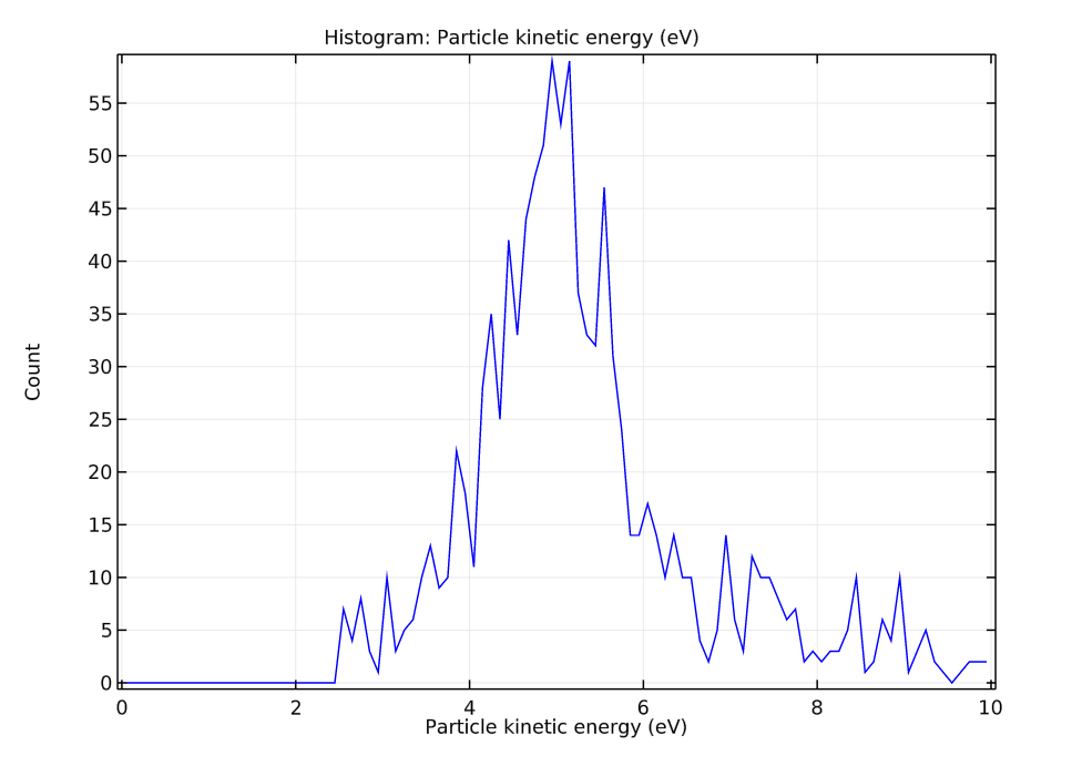
Note that the last line is just Eq.(3). The following plot is a histogram of the value of rn for a population of 1000 particles. The smooth curve is the exact Rayleigh distribution, which has been defined using an Analytic function feature.
![Graph plotting the histogram of sampled values against the exact Rayleigh distribution.]()
For curves with many fine details, a larger number of particles may be needed to accurately capture the probability distribution function.
Note About Interpolation Functions
If a probability distribution function is entered into COMSOL Multiphysics as an Interpolation function feature, instead of an Analytic or Piecewise function, then you can use built-in features to automatically define a random function that samples from the specified PDF.
Suppose we have an interpolation function that linearly interpolates between the following data points:
|
x
|
f(x)
|
|
0
|
0
|
|
0.2
|
0.6
|
|
0.4
|
0.7
|
|
0.6
|
1.2
|
|
0.8
|
1.2
|
|
1
|
0
|
The following screenshot shows how this data can be entered into the Interpolation function. By selecting the Define random function check box in the settings window for the Interpolation function feature, you can automatically define a function rn_int1 that samples from this distribution. In the Graphics window, the histogram plot shows a random sampling of 1000 data points, and the continuous curve is the interpolation function itself. The extra factors 20 and 0.74 are included to correct for the number of bins and normalize the interpolation function, respectively.

The Power of Probability Distribution Functions
So far we’ve seen how probability distribution functions, cumulative distribution functions, and their inverses are related. We’ve also discussed several techniques for sampling from both uniform and nonuniform probability distribution functions in COMSOL models. In the next post in our Phase Space Distributions in Beam Physics series, we’ll start explaining the physics of ion and electron beams and how an understanding of probability distribution functions is essential to accurately modeling beam systems.
References
- Humphries, Stanley. Charged particle beams. Courier Corporation, 2013.
- Davidson, Ronald C., and Hong Qin. Physics of intense charged particle beams in high energy accelerators. Imperial college press, 2001.


")


")
")
")
")


 that is also on the line, then a fourth point
  , and so on, and thus infinitely many distinct points can be obtained. This is illustrated below.
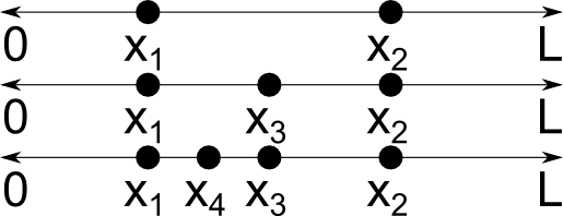

 . Let’s look at an example in which this method is used to sample from a nonuniform probability distribution function.


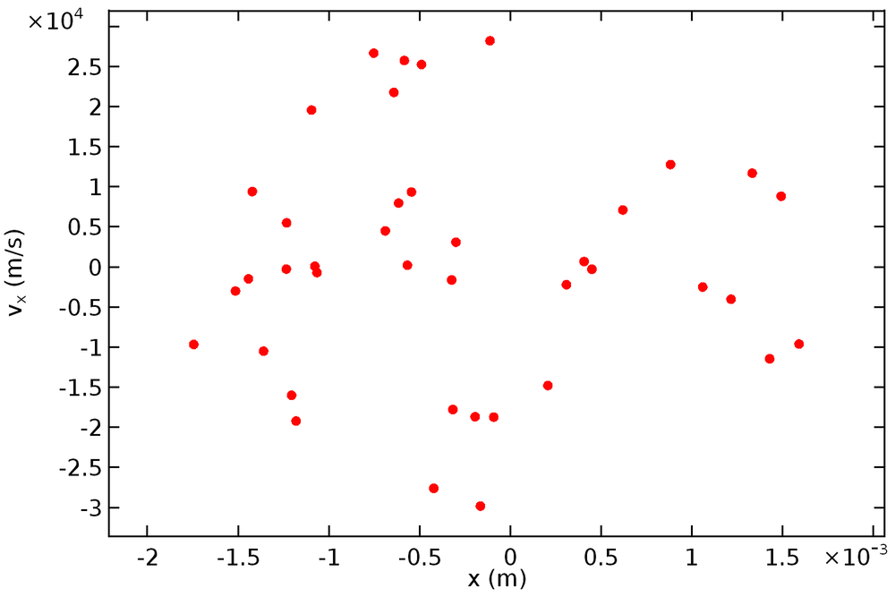
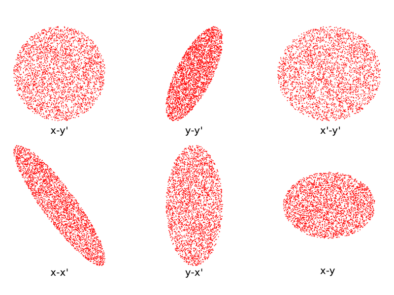
 . (It’s fair to call this quantity an angle because
  in the paraxial limit.) The distribution of x and x’ values of particles in the beam is the trace space distribution, and the ellipse that encompasses this distribution is the trace space ellipse.
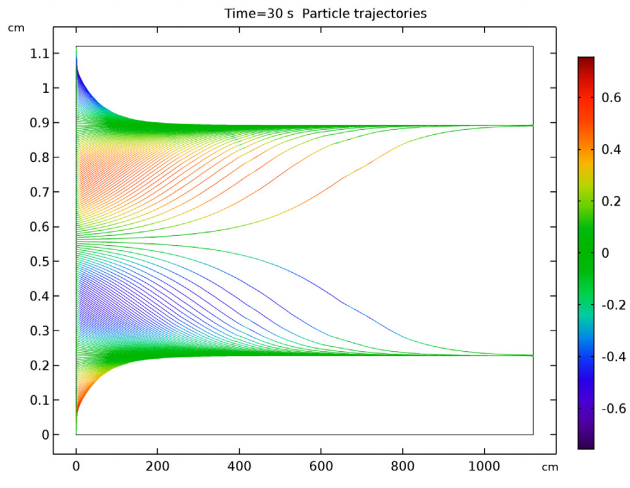
 . Similarly, particles with negative transverse velocity will move to the left. The following animation shows the evolution of a phase space ellipse over time for a drifting beam without space charge effects.
 is also called the Courant-Snyder invariant.
 ) and Eq.
 and
and  .
.